Dear Reader: This is the fourth in a series of articles on using the unemployment rate (U) for commercial loan loss forecasting, including CECL and stress testing. In the first three posts, we described how industry-wide C&I charge-offs (C&I COs) lead the unemployment rate and how, unlike with most consumer loans, C&I charge-offs trail defaults, on average, so the unemployment rates lag defaults even more. We also offered for a few of the reasons why banks use unemployment for C&I loss forecasting.
In this article, we look at the relationship between the same national unemployment rate and the banking-industry-wide Commercial Real Estate loan charge-offs (CRE COs or just, plain COs, depending on the context). As with C&I, we analyzed both seasonally-adjusted (SA) sequences, which are the ones usually seen or presented, e.g., the Fed’s CCAR scenarios use seasonally-adjusted numbers, as well as raw, non-seasonally adjusted sequences. Here, we’ll present both as there are slight differences in timing that are worth showing.1
Alas, our results are similar to the C&I case: CRE charge-offs lead the unemployment rate.
As with C&I, we start with time series graphs:


Notice that on both the seasonally-adjusted (SA) and non-seasonally-adjusted (NSA) graphs, peaks in the unemployment rate never precede peaks in CRE charge-offs. In fact, in the NSA or raw or real case, CRE charge-offs peak earlier than unemployment. In both, there is a false positive; there is a rise in the unemployment rate in 2003, but no corresponding increase in CRE charge-offs. Particularly for risk management purposes, which should include all of stress testing, we’re baffled why firms (and the Fed) use only seasonally-adjusted numbers, and, at a minimum, don’t investigate the raw series. (Banks don’t seasonally-adjust PDs, LGDs or EADs when building loss-forecasting models models.) Granted, the lines are smoother and prettier but less representative of the most interesting—read extreme—cases. As an analog, consider a river or lake that is dry for six months and 20-feet-deep for six months. We don’t want to break our neck diving into a dry bed that has a seasonally-adjusted depth of ten feet. Similarly, if something bad happens when a customer’s quarterly cash flows and financial position are at their weakest, we don’t want to average away that worst case.
Now, back to CRE. Let’s eliminate the time dimension, and consider the relationship between U and CRE COs, via scatter plots.
However, rather than show contemporaneous observations as we did with C&I, here, we’re showing pairs with charge-offs at time t and the unemployment rate at time t + 2 (as that lag/lead seems to reveal the strongest relationship).2 The inverse, with CO on the horizontal access, is the second slide.


Notice the two distinct regimes. As with C&I, the differences relate to The Financial Crisis, albeit with slightly different cut-offs: pre and post Q2/Q3 2008, with observations from 1991 – Q2 2008 in purple and Q3 2008 – 2019 in green.
It’s rare to see such strong, clear relationships. With U on the horizontal axis, both appear to be convex—although as with C&I, the earlier regime seems to have less curvature. For regression analysis, it would be possible to shift the curves sideways and have a larger sample set and try to find one relationship. In fact, it’s easy to imagine inexperienced or otherwise clueless developers doing just that; however, “possible” doesn’t mean “advisable.”
There are two distinct relationships within the sample history, and they shouldn’t be ignored, (Like all empirical results, whether the latter relationship continues into 2020—we doubt it will—is an example of the Problem of Induction, which philosophers and others having been contemplating for millennia.) Again, and intuitively, if the graphs illustrate such nice “average” relationships with CRE COs leading U by two quarters, there’s a pretty good chance this will be observable in the correlations.
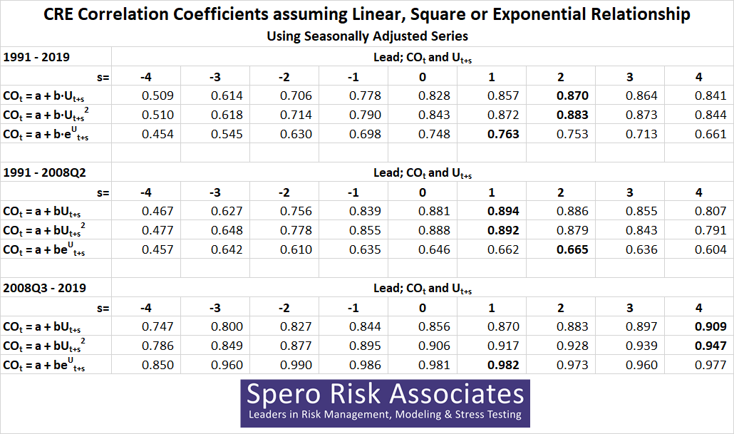
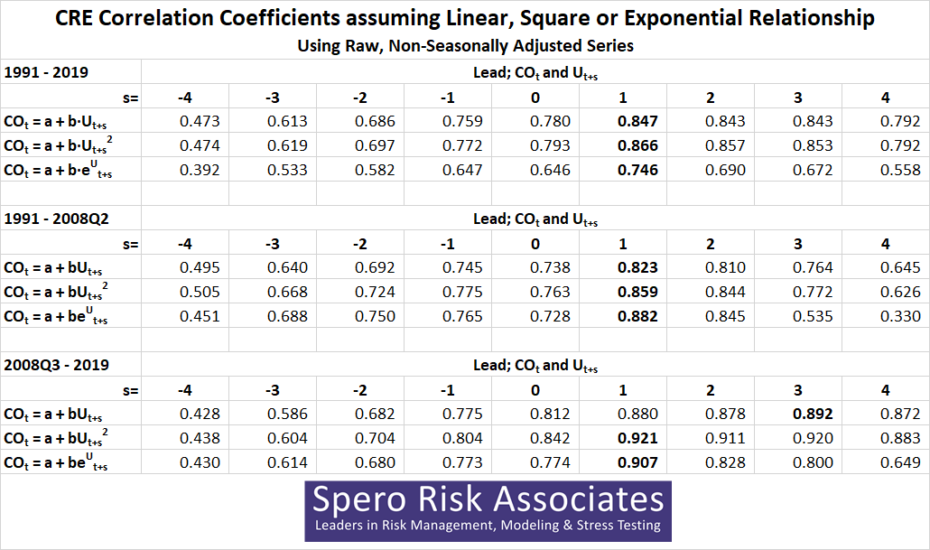
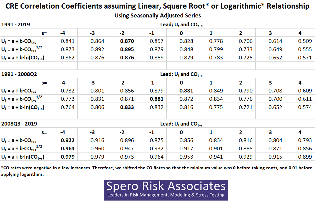
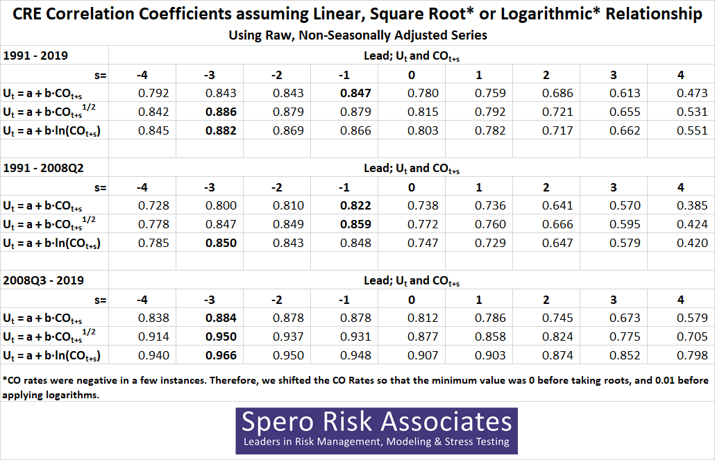
As with C&I, we present correlations for three cases—no transformation, square (or square root) and exponential (or natural logarithmic)—for the whole sample history and for each of the regimes. We make no claims that any of the three provides the absolute best fit, but all serve our rhetorical needs; regardless of the transformation applied, the highest correlations are found when CRE charge-offs lead the unemployment rate—usually by one or two quarters. There are four tables in the slider: CO as the dependent variable—both SA and NSA—and U as the dependent variable—both SA and NSA.
- Contact us if you would like more information. All data sequences that we’re using are free and public from FRED. ↩
- We’re also showing the SA sequences, as they’re prettier, but the NSA plots at various leads and lags are available upon request. ↩