This is an article about economic regimes—particularly credit regimes—and living inside one (which you always are). The biggest issue you face is not appreciating that fact or its implications. Fortunately, once noticed and identified, pretty much the only risk that matters can be measured and managed.
Good Times, Bad Times
What do we mean by a “regime?”
We mean an environment, market, or industry where periods of calm—sometimes long periods of calm—are interrupted by seemingly sudden and intense turbulence and loss; we’ll call that sudden change a “deluge,” and since we’re focused on credit, we’ll refer to one as a “credit deluge.” With regimes, loss rates are bimodal; so, the average loss rate across all time doesn’t represent any particular time; it’s a number between a very low rate and a very high one. For example, our average, good-time, net charge-off rate for bank-industry CRE is 6 bps versus a historical average of 46 bps and a bad-time average over 1%.1 If you want a natural analog, it’s like a river that’s dry or low most of the year but occasionally floods—quickly or massively. The average—seasonally adjusted—depth is only measured when the water rising or falling; so, knowing that isn’t very useful for planning purposes, because knowing the long-term average doesn’t help determine whether you should walk or swim across it.
In good times your portfolio can absorb defaults and the subsequent low losses associated with idiosyncratic borrower or loan problems. That’s what makes them good times, after all! Excluding fraud, you won’t lose much, because either (1) your collateral’s value is likely to have remained high—think rising house prices—or (2) for, say, an unsecured business loan, someone else may want to give the business a try or at least buy the assets to use elewhere.2 In bad times, neither tends to be true… and you’re stuck with stuff that nobody wants at exactly the worst time.
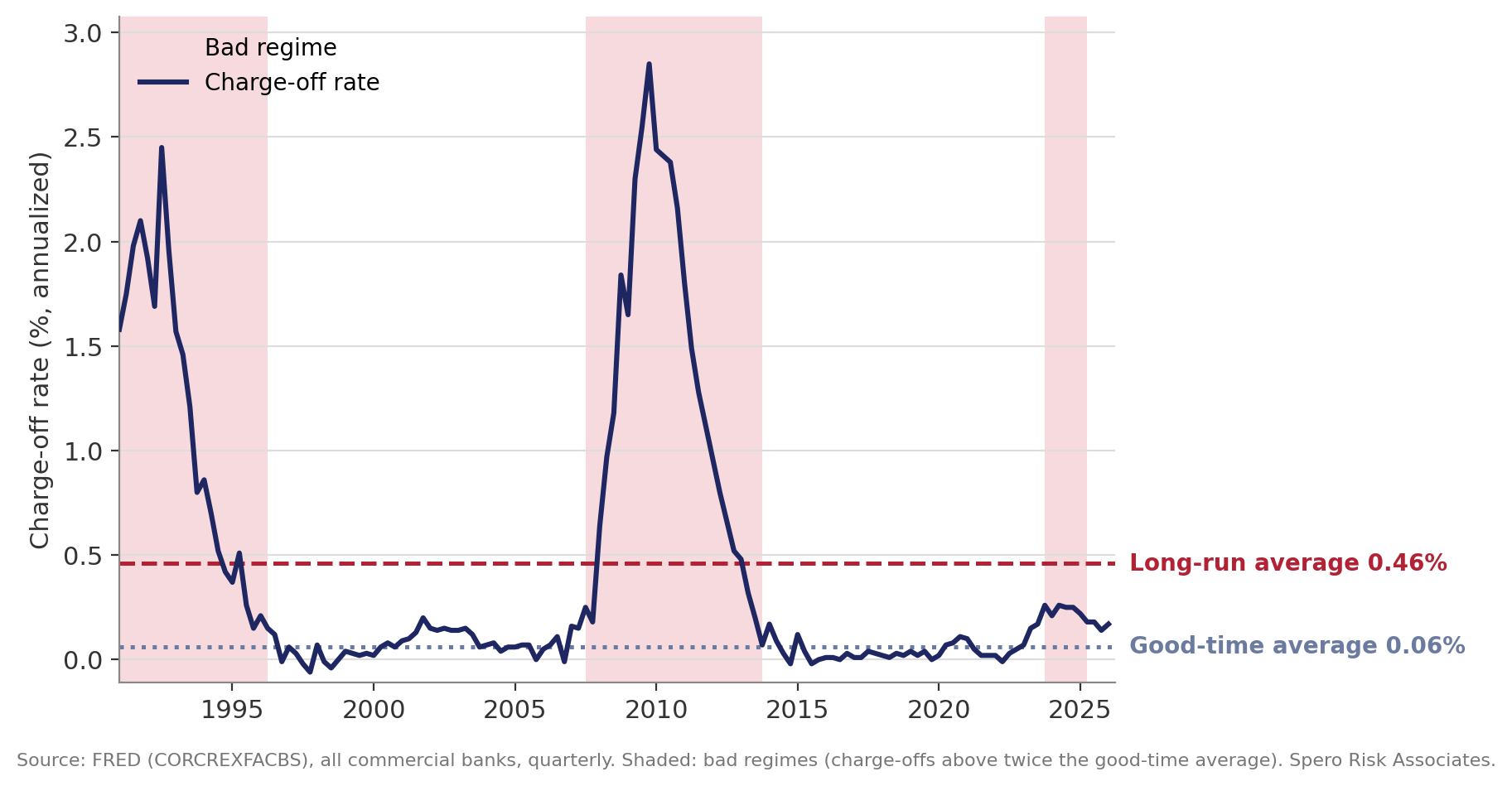
Commercial real estate charge-off rate, all commercial banks (FRED: CORCREXFACBS), with its long-run and good-time averages. Shaded areas are bad regimes.
Running the Wrong Race
Credit modelers—implicitly or explicitly—often use a competing hazards approach for loss forecasting. What’s that? That’s just a fancy way of saying there is a race between pay-off (usually good) and default (bad, but in good times, usually not too bad). Some modelers spend a lot of time and effort on getting the two rates right across borrowers, times, and (some) conditions. It’s useful work, but it’s not the race that really matters, because, as the graphs show and as we’ve mentioned, the preponderance of losses occurs in bad times: for residential mortgages, ~80% of cumulative losses occur in ~20% of the quarters, and those quarters cluster together. Take a minute to consider that: ~80% of cumulative losses occur in ~20% of the history. (When you see such numbers, here, note that for comparability, we’re holding balances constant through time, which seems like the right thing to do.) The problem with focusing on the race within the race during good times—where 80% of the observations lie—is that it can obscure the race will bigger consequences. That’s the 80% of history that doesn’t tell you much.
Heck, for most portfolios, you can substitute a good-time loss rate, like our 6 bps above—or a set of good-time loss rates conditioned on borrower and loan characteristics—for a model and lose very, very little. In fact, if you have a strategic perspective, you’ll realize that you’re usually losing nothing—literally AND figuratively. Look at the graph above or the resi one below; the averages in good times would suffice as a quarterly loss estimate… in good times. Averaging that good-time rate with the bad-time rate tells you very little, and that can be a big problem for stress testing, where developers always want more observations for their statistical tests but not necessarily the right observations (to understand how and when most of the losses arise). Reverse our numbers above: ~20% of resi’s losses occur in ~80% of the history. And a statistical fit counts observations, not losses. If you pool the regimes, the good times get ~80% of the weight in the estimates—and in the tests of the relationships—while producing only ~20% of the losses. More good-time observations aren’t going to help estimate the losses you (should) care about.
Pro tip: Resources are limited. Spending the money on re-estimating models to change the good-time estimate (by a basis point of a basis point when your good-time losses are, at most, basis points) means you’re not spending it on identifying the conditions that could accelerate the arrival of bad times or make their consequences (full percentage points, not basis points) worse.
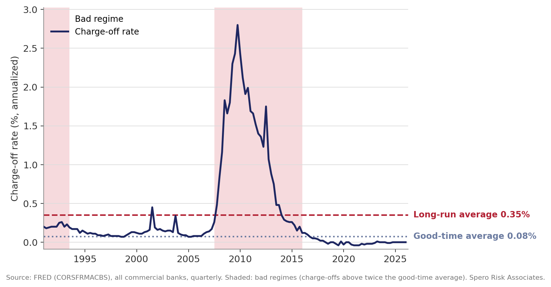
Residential mortgage charge-off rate, all commercial banks (FRED: CORSFRMACBS), with its long-run and good-time averages. Shaded areas are bad regimes.
How Low Good-Time Losses Lead to High Bad-Time Losses
Regimes—whether credit, interest rate, or whatev—are everywhere, all the time. Ecclesiastes (3:1) knew it, as did those who lived along the Nile and the Euphrates thousands of years ago. Nile floods were so predictable that Egyptians based their calendars on their arrival. Credit deluges are more like flooding on the Euphrates; the intervals aren’t as certain. What is certain is that they’ll occur, and they’ll be costly.
What is inescapable is that 20 or even 50 years of evidence doesn’t preclude the possibility of, or damage from, a 100-year flood.3
Likewise, 15 years of low loan losses doesn’t preclude a credit deluge that is the start of bad times. Those bad times tend to generate losses that are nearly two orders of magnitude (>50x) greater than the minuscule loss rates observed in good times. As we mentioned above, total losses during shorter, bad times are multiples of total losses during longer, good times. For example, CRE losses in bad times are 7–9 times those of good times, and that’s despite the fact that good times last 2.0–2.5 times as long.4
The reader might argue that our use of “doesn’t preclude,” above, is very different than “will cause.” Indeed! That’s true, but that doesn’t mean that nothing can be known about the conditions that accelerate a deluge’s arrival or its consequences. Let’s be clear: we don’t know when a deluge will occur, and never claim that we do. Permabears make the claim—like the guys who stand on a street corner shouting, “Repent! The end is nigh!” for years and years and years. What we do know is that deluges are not just possible, they’re inevitable, and they’re more likely to arrive sooner and hit harder under certain conditions, including:
- Believing that we—our glorious generations—are at the end of history. Yeah, it may be different this time, but not that different. We have not eliminated risk. It’s not even clear if we understand it better. Maybe we hide it better or unintentionally obfuscate it and then take comfort in not seeing it.
- Here’s the catch: not knowing that you’re in a good regime, or knowing but exempting yourself from history and the inevitability of a regime change, alters your behavior and decisions. If good times are the new normal, then loosening standards can look smart. To see that, consider what the decision becomes. Let’s set funding costs to zero so we can ignore them. In that case, in good times, looser credit standards generate marginal expected interest revenue that exceeds (short-term) marginal expected credit losses; so, short-term profits may increase. Using that as evidence that lending lower down the borrower quality scale is safe is like standing in a dry river bed, noting that it seems to never rain here, and then deciding to build your house lower on the bank. Why not? The land is cheap, too!
In good times, you may not notice that marginal borrowers have less margin, less cushion, like the private credit borrowers or ARM holders who can’t withstand an interest rate shock. In calm, good times, looser standards raise the probability of default only slightly, and as we noted above, when a loan does default, you can usually offload it with little loss. Look at those graph: net charge-off are negative a decent amount of time within the good regimes.
The question is what happens in the long term, where “long term” includes a deluge with an uncertain start date, followed by bad times of uncertain severity? That is the real race:
Will you get paid back before the deluge hits the fan?
For the moment—and only for the moment—let’s ignore the fact that lenders’ loosening actions during a period of prolonged calm will likely accelerate the arrival of bad times and increase their severity and maybe their length, but we’ll get back to that. (Just forget that for now.) Even without those compounding factors, you’ll lose quite a bit more in bad times. Marginal borrowers and projects don’t have the wherewithal to survive hard times, and if you (and others) have loosened standards, when conditions change, those weak customers will be hit hard by the environment and fail at higher rates than creditworthy ones. That’s the direct effect, and no different than building far down on the river bank because it’s been dry for so long.
The indirect effect is the major difference between our river analog and lending. When you relax standards, more marginal projects are funded. It’s indirect but perfectly predictable. In isolation, lending to one marginal borrower might not matter much, but if you do it, and everyone else does it, and your marginal borrowers transact amongst themselves or with your peers’ marginal borrowers, then a small ripple of inconvenience near one can become a tsunami of despair. That’s what you learned in integral calculus: a bunch of nothings can become something.
In fact, even otherwise sound borrowers can become marginal during good times. How? In one of two ways:
- If they have an expanded or large customer base of marginal—and now failed—firms, the old stalwarts become riskier.
- Under certain conditions, like low interest rates and ample liquidity, highly-rated credits may be tempted to invest in marginal projects they’d never have considered if money were scarcer… thereby making themselves less creditworthy—even though their track records to that point say otherwise.
What we’re describing is known as the “cascade” effect and percolation. The cascades aren’t accidents. They’re collisions with foreseen consequences. So, congratulations! Marginal-loan-by-marginal-loan, the industry has created systematic risk during good times. That’s how lending differs from our river metaphor: building lower doesn’t increase the chance of rain and a flood. Lending lower does.
So how does anyone talk themselves into believing that the past is irrelevant—and we do it all of the time—and it’s different this time? Let’s visit the Oracle at Delphi for an illustration.
Private Credit: Our portfolio is pristine. Isn’t it? Loss rates are in the single basis points. We can’t lose, can we?
The Oracle: Your leveraged loans are the same as the banks’ in 2006, when they had single-basis-point losses. A few years later, they lost 80–90 times that rate.
Private Credit: No, it’s different this time. We’re not banks.
The Oracle: Oh, okay!
(To herself: Let’s see how that works out for you.)
Our readers wouldn’t be fooled so easily. They would want to know, “What can be done in good times to mitigate the harmful effects of bad times?”
What Should You Do?
Think of it as the five stages of grief, worked through before the loss instead of after.
1. Denial: good times won’t last forever.
Suffer neither myopia nor tunnel vision. Realize that your actions and decisions—however small—have their own long-term effects, and they can combine with others’ actions to hasten the arrival and increase the severity of a deluge. Recognize that your long-term planning horizon must include a deluge.
2. Anger: don’t blame others; learn from them.
Times do change, e.g., unprecedented low rates and liquidity, but not that much; there are always marginal borrowers who can do real harm. Don’t look for reasons why the past is irrelevant. Look for reasons why it’s relevant. Don’t throw out the lessons of the past because there isn’t enough data from the time to build a model. (For a short list of repeat failures, see the appendix.)
3. Bargaining: ask “what if?”—and measure the answer.
That involves serious stress testing.
What do we mean by “serious?” For larger organizations, CCAR may be a necessary regulatory exercise, but it’s not sufficient. CCAR is nine quarters. Starting in 2007 and depending upon how you measure the regimes, the bad times lasted for 6.0–8.5 years, 5.0–6.0 years, and 4.5–5.0 years for resi, CRE, and C&I, respectively. The minimum of those regimes was 18 quarters, twice CCAR’s nine quarters. In fact, at best, CCAR’s nine quarters would only capture 32–40%, 35–51%, and 44–59% of GFC-related charge-offs for resi, CRE, and C&I, respectively.5
For those three portfolios, here’s a look at major downturns since their series, available at FRED, began. Note CCAR’s nine quarters only capture mild cases. That’s not “severely adverse,” by any definition.
| Portfolio | Bad regime | Length | Losses inside the first nine quarters |
|---|---|---|---|
| Residential | 1991–1993* | 2.5 yrs | 89% |
| Residential | 2007–2015 | 8.5 yrs | 32% |
| CRE | 1991–1996* | 5.2 yrs | 69% |
| CRE | 2007–2013 | 6.2 yrs | 35% |
| C&I | 1989–1992 | 3.2 yrs | 73% |
| C&I | 2001–2002 | 1.0 yr | 100% |
| C&I | 2008–2012 | 4.5 yrs | 59% |
A bad regime is a stretch when charge-offs run above twice their good-time average. *The residential and CRE series begin in 1991, in the middle of these episodes, so they were longer than shown. The last column assumes the nine-quarter window starts on the first quarter of the deluge, which is the best case.
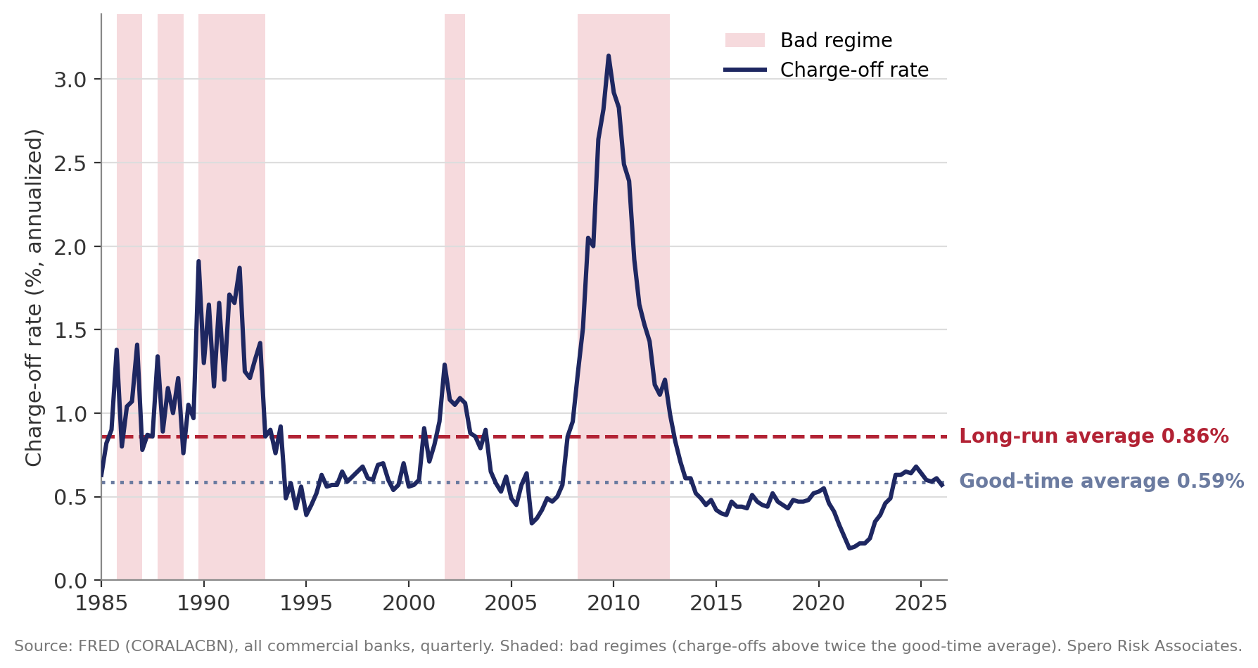
Commercial and industrial loan charge-off rate, all commercial banks (FRED: CORALACBN), with its long-run and good-time averages. Shaded areas are bad regimes.
So, one concrete action is to set your forecast horizon for each portfolio equal to the average length of its stress periods. If you want to be conservative, choose the maximum length (all observed in the GFC). That’s a marginal improvement, not a fundamental one.
4. Depression: understand depressions. Use loan-level stress tests differently.
An expanded stress test is better but not great. The solution does involve loan-level stress tests… but used in a creative (and once shown, obvious) way to identify the long-term implications that through-the-cycle averages and other “long-term” risk management metrics ignore, hide, or obfuscate.
- CECL reserving doesn’t capture it.
- Typical stress testing doesn’t capture it.
- Vintage/TOB analysis doesn’t capture it.
- Economic Capital doesn’t capture it. Trying to find a one-in-a-thousand-year loss with 20 years of data—think dry river bed—doesn’t capture anything except The Politician’s Fallacy.
- Traditional portfolio management methods don’t capture it.
- Model validation and back-testing in good times—where even a fixed, conditional average tests well—don’t capture it.
- Risk ratings and credit scores, either point-in-time or averaged through-the-cycle, don’t capture it.
- RAROC and pricing to one-year expected loss don’t capture it.
- ALM and credit, run separately, don’t capture it. That’s how private credit borrowers could default in the fourth year of a loan, after their three-year rate caps expired. A change in the environment that no one considered.
Each function, each metric does something; it provides a facet—a narrow, assumption-laden perspective. Individually and collectively, they’re insufficient to identify the risk that kills— the wave. If you know the old analogy of the blind men and the elephant, then each method touches a real part of the elephant. None of them sees the elephant. Failing at nothing. Failing at everything by not managing the one risk that matters the most.
So, what do we have? First, note that it’s impossible to manage any portfolio without knowing how, where, when, who, and why you could lose money. Without those facts, there’s no way to tell which positions to add and which to cut. We’ve shown that across the three portfolios, most (~75%) historical losses arrive in the deluge; so, your risk management should be built around the deluge. Day-to-day tasks are necessary, too, but they’re probably built around good times and the (smaller) risks seen there. Managing risk in the next quarter is easy; it’s too late to do anything. So, action becomes reporting and reports emphasize the short term and that becomes a cycle. You should be managing for the next deluge, not the next month-end or quarter-end.
5. Acceptance: the loss is coming. Measure it now.
All of this can be done with the loan-level data you may already have. Why loan-level? It’s the only way to identify your truly marginal loans: the 20% of borrowers who will generate 80% of your losses in bad times… which are 80% of your historic losses. A fifth of your loans, in a fifth of the time, produce nearly two-thirds of everything you’ll ever lose. That seems like something to think about!
The rest is standard risk management: (1) identify, (2) measure, and (3) act today or plan now on how to act when the deluge arrives.
That doesn’t require knowing when the deluge will come. It only requires admitting that it will.
A trade-off to consider: tightening (or not loosening) standards in good times costs you something visible every good quarter: the spread on the marginal loans you don’t make. What it buys is substantially less tail risk when the deluge arrives, and there are specific, precise methods to measure that risk. In a crisis, your losses will be substantially lower—not the two-orders-of-magnitude increase that some others will see—and you’ll have the capacity to lend and buy when others can’t. It reminds us of Kipling’s “If—”: If you can keep your head when all about you / Are losing theirs and blaming it on you… If you can meet with Triumph and Disaster / And treat those two impostors just the same… If you can wait and not be tired by waiting…
The goal isn’t the best return in good times. It’s the best return when the deluge is counted. So, either you can count it, or it will count you… among its victims. You can measure the costs and benefits of discipline and make the case to your board and investors in advance. Agreed upon beforehand, the opportunity cost, which may appear to the uninformed as good-time “underperformance,” is just an insurance premium. Measured that way, the lender who tightens (or doesn’t loosen) doesn’t underperform; the others just hadn’t been billed yet. When the bill does come due, it looks like they stayed in the house that everyone knows they should have left. (Is that a chainsaw we hear?)
6. Contact us.
If it’s not already clear, yes, we know what to do, and how to do it in the most cost-effective way. To learn more, contact us.
Appendix: That Was a ‘Them’ Problem, Not an ‘Us’ Problem
Maybe, but probably not.
We’re planning a long article on the repetitive nature of regimes across the years, decades, and centuries, but here is a short list.
The S&Ls weren’t the thrifts that got destroyed in the rate shock, and they were right about that. The old model—thirty-year fixed mortgages funded with passbook savings—really had been killed by Paul Volcker’s rate shocks, and everybody knew it. Deregulation handed them commercial real estate, junk bonds, direct equity stakes, and brokered deposits to fund it all. They called it diversification. They should have called it a minefield. What they had actually done was trade a rate-risk problem for a credit-risk problem… in asset classes they had never underwritten… with a regulator that had never overseen any of it.
1998 wasn’t a mania. It was convergence arbitrage, run by people who had won the Nobel Prize for the math. Heck, the positions were hedged: go long the cheap instrument, go short the rich one, and collect when the spread closed. That’s what justified the leverage; thirty times isn’t a big deal if you’re not taking a directional bet, right? Then Russia defaulted, every spread widened at once, and it turned out the long and the short legs were the same trade. The “hedge” was actually a correlation assumption dressed like a hedge.
Telecom in 2001 wasn’t the dot-coms, and the distinction was real. Dot-coms were websites with no revenue; this was conduit, switches, and transoceanic cable—built by companies with actual contracts, financed with actual high-yield debt. Everyone cited the statistic that internet traffic was doubling every hundred days, but… nobody checked it, and… it wasn’t true. So, capacity became several multiples of demand, and it turned out that fiber in the ground is worth roughly nothing if there’s no traffic to put on it. (Reminds us of the old 19th-century plank roads. Also reminds us of something else. What could that be?)
Subprime wasn’t the S&Ls, because the risk didn’t stay in one place. The broker got paid at the closing table, the aggregator got paid at the sale, the trust got paid at issuance, and the tranches went to somebody who would never meet the borrower. Everybody in that chain was underwriting the next transfer, not the loan itself. Let’s drop the notion that this was a fraud committed by borrowers. If you write it, they will come; stated-income lending was a product category, pushed because loans closed faster and were priced better, and the 2/28 with a teaser reset was underwritten to a future refinancing rather than to payment. (Pro tip: not a good idea.) The loan was designed to be replaced before it became a problem. That works fine as long as somebody is there to replace it or buy the house.
Private credit isn’t leveraged-loan banking in 2006. It’s senior secured, sponsor-backed, covenanted, held to maturity by “patient capital” that doesn’t have to sell into a bad tape. The floating coupon is described as protection against rising rates, which it is—for the coupon—but not for the borrower. The borrower has no such protection, especially the marginal borrower who doesn’t buy (can’t afford) interest rate protection and can’t absorb a rate increase. It’s just a coincidence that bank loss rates pre-Crisis are similar to PC loss rates pre-current situation, right? PC’s low loss rates have nothing to do with extending-and-pretending otherwise severely delinquent loans, do they? (BTW, does PC even have collections departments? Won’t that affect LGDs?)
Credit insurance and CDS (credit default swaps) weren’t the mortgage guarantee companies of the 1920s and early ’30s. Those offered a 5% coupon guaranteed by a large title or insurance company—no models, just the guarantor’s word. The 2006 versions had models! And AAA ratings! And AIG insured only super-senior tranches! (The ones that couldn’t be reached.) The 1920s guarantors pooled mortgages they had guaranteed, put them in trusts, and sold shares in the pools to ordinary investors: a pass-through with a guarantee, eighty years early. The business kept growing into 1930, on a decade in which rising prices had let defaulted properties be sold without a loss. (Defaults without losses. Sound familiar?) But prices fell about a quarter between 1928 and 1933, and in August 1933, New York seized fourteen companies in one month. By the end of the year, nobody was guaranteeing mortgages. The answer, in 1934, was the FHA. Which brings us to our next depressing entry…
FHA isn’t subprime: every loan is full-doc, every income verified, every borrower underwritten. No liar loans here! That’s all true, and it’s all beside the point. About 7.05% of FHA mortgages issued in 2024 went seriously delinquent within twelve months, compared with 7.02% for FHA’s own loans at the 2008 peak.6 So recent FHA loans perform as poorly as FHA loans did near the peak of the Crisis. The better comparison, though, is with subprime loans before the Crisis. The best we can tell, and shockingly, subprime vintages from 2003–2006 performed better in their first 12 months—sometimes much better—than recent FHA loans have. That changed in 2007, when they performed worse, but that was the start of the Crisis.7 So: worse performance, but with honest paperwork. It’s the same people who couldn’t afford the house—just a generation removed. Loan-to-value (LTV) determines the severity, not the quality of the borrowers’ documents (even if they’re notarized!), and 3.5% down is 3.5% down. Turns out that 3.5% down isn’t very much. The documentation problem was fixed. To what end? (Oh well, it’s only the taxpayers’ money! More precisely, their great-grandchildren’s.) Oh well, those houses are concentrated in other neighborhoods—who cares about the collateral damage of the exploding loans? Home prices will recover, right?
Crypto is new! It’s not like tulips! Nothing like it before! It’s spent electricity! It’s new in the sense that you can’t grow it and enjoy it for a week or so, like a tulip.
The Tulip Bulb mania of 1637 seems silly to us sophisticated, modern types because it was so obviously silly: everyone knows what a tulip is. Our examples since the 1970s are the same errors, just better hidden, because we’re all so sophisticated nowadays. Who could have known?
Subprime and FHA early defaults (footnote 7). Share of loans in default 12 months after origination. Subprime: Mayer, Pence, and Sherlund, “The Rise in Mortgage Defaults,” Federal Reserve FEDS 2008-59, Figure 2 (figure data). FHA 2024: Allysia Finley, Wall Street Journal, February 23, 2025 (90+ days seriously delinquent within twelve months; comparison approximate).
| Vintage | In default 12 months after origination |
|---|---|
| Subprime 2004 | 1.7% |
| Subprime 2005 | 2.8% |
| Subprime 2006 | 5.8% |
| Subprime 2007 | 9.3% |
| FHA 2024 | 7.05% |
Sources: Charge-off series from FRED: CORSFRMACBS (residential), CORCREXFACBS (CRE ex-farmland), CORALACBN (C&I). Regimes, lengths, shares of losses, and nine-quarter capture rates are Spero Risk calculations, using two definitions of a bad regime (charge-offs above their long-run average, and above twice their good-time average). Peak-to-calm ratios, 2004–06 average to 2009Q4 peak: CRE 51x, residential 31x; against the lowest non-zero quarter, both approach 280x. FHA: Allysia Finley, Wall Street Journal, February 23, 2025. Subprime vintages: Mayer, Pence, and Sherlund, Federal Reserve FEDS 2008-59. Rasuwa, Nepal flood of August 26, 2026: flood-wave speed from Jeffrey Kargel, Planetary Science Institute, as reported by CNN. Scripture quotations: NABRE. Related posts: Credit Regimes, Risk Management, and the Value of Stress Testing; Are Banks Ready for a Downturn?; Was Private Credit Fooled by Its Own Success?